After studying this material, you should be able to:
- Explain why graph query serving layers require distinct design decisions from ingestion and storage layers
- Compare shallow-wide vs deep-narrow query patterns and their respective challenges
- Justify key architectural choices: breadth-first traversal, async execution, selective caching, and opt-in enrichments
- Trace a multi-hop query end-to-end through the three-layer architecture
- Apply filtering hierarchies and concurrency control concepts to real distributed system design problems
Step-by-Step Study Material
Step 1: Understanding the Problem Space
Why Querying is Its Own Challenge
Think of building a library system. Acquiring books (ingestion) and organizing shelves (storage) are hard problems. But helping someone find exactly what they need quickly is a completely separate challenge.
Netflix's RDG faces the same separation:
Ingestion Layer → Storage Layer → Serving Layer
(Apache Flink)    (KVDAL)         (THIS article)
The serving layer must answer:
"How do we turn a billion-edge graph into sub-100ms responses?"
The Two Extremes of Query Patterns
Before designing anything, Netflix identified that queries fall along two axes:
         DEPTH (hops)
           │
    Deep   │  Deep-Narrow
           │  (few nodes, many hops)
           │
           │
  Shallow  │  Shallow-Wide
           │  (many nodes, few hops)
           └──────────────────── WIDTH (fan-out)
              Narrow        Wide
Example 1: Shallow-Wide Query
"Which devices has this account used in the last 30 days?"
Account X ──streamed_from──► [Device1, Device2, Device3... Device500]
           (1 hop, massive fan-out)
Challenge: Fetching hundreds of edges, applying time filters on each, aggregating results — all under 100ms.
Example 2: Deep-Narrow Query
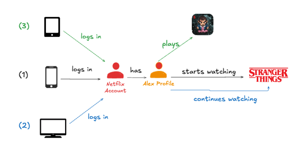
"Show me Stranger Things viewing history across all profiles for Account X"
Account X ──has_profile──► [Profile_Alex, Profile_Kids]
                                    │
                           started_watching
                                    │
                                    ▼
                           [ST Season 1, ST Season 2, ST Season 4]
Challenge: Sequential dependency — you cannot fetch viewing history until you know which profiles exist.
Why Sequential Dependency Hurts
Without optimization:
├── Hop 1: 10ms network time
├── Wait for Hop 1 to complete
├── Hop 2: 10ms network time
├── Wait for Hop 2 to complete
└── Total overhead: 20ms+ before processing a single byte

With 3-4 hops: 30-40ms of pure waiting
Key Insight: These two patterns pull the system in opposite directions. Shallow-wide stresses I/O throughput. Deep-narrow stresses execution efficiency. The design must handle both simultaneously.
Step 2: The Five Core Design Decisions
Each decision answers a specific problem. Understanding the why is as important as the what.
Decision 1: Breadth-First, Not Depth-First Traversal
Depth-first (intuitive but wrong for distributed systems):
Account X
└── Profile_Alex
    ├── ST Season 1 ← finish this entire path first
    ├── ST Season 2
    └── ST Season 3
└── Profile_Kids ← only then start here
    └── ST Season 4
Breadth-first (counterintuitive but correct):
Level 1: Fetch ALL profiles simultaneously
         [Profile_Alex, Profile_Kids]
                    ↓
Level 2: Fetch ALL viewing histories simultaneously
         [ST S1, ST S2] + [ST S4]
Why it matters:
| Approach | Network Calls | Parallelism |
|---|---|---|
| Depth-first | Sequential per path | None |
| Breadth-first | One round per level | Maximum within each level |
Trade-off: Breadth-first holds an entire level in memory at once. Netflix manages this by bounding each hop with per-edge-type limits (covered in Step 5).
Decision 2: Async-First, Not Thread-Per-Request
The problem with thread-per-request:
Traditional Model:
Thread 1: [Processing]──[WAITING for storage]──[Processing]
Thread 2: [Processing]──[WAITING for storage]──[Processing]
Thread 3: [IDLE]──────────────────────────────────────────
...
Thread 1000: [IDLE]

Result: 1000 threads, most doing nothing
Async model:
Async Model (16-24 threads total):
Thread 1: [Query A]──[start storage call]──[Query B]──[Query C]──[Query A result arrives, resume]
Thread 2: [Query D]──[start storage call]──[Query E]──[Query D result arrives, resume]

Result: Same threads handle thousands of concurrent requests
Real-world impact: A serving layer that would need hundreds of threads per instance runs on just 16–24 threads.
Trade-off: Async stack traces are hard to debug. Netflix compensated with per-stage metrics at validation, storage, enrichment, and end-to-end stages.
Decision 3: Selective Caching, Not Cache Everything
The volatility spectrum:
STABLE (cache with long TTL)          VOLATILE (don't cache)
│                                              │
▼                                              ▼
Account plan type                    "Who watched what, when"
Content metadata                     Real-time edge data
Profile attributes                   Recent activity edges
Smart TTL Policy:
Node last active: 99 days ago
Graph retention window: 100 days
Node expires from graph: tomorrow

→ Caching with 30-day TTL = WASTEFUL
→ Skip caching entirely
Result: 70–80% cache hit rates by being selective, not aggressive. This translates to roughly 3–4x fewer storage calls on common query paths.
Decision 4: Opt-In Enrichments, Not Automatic
The problem with automatic enrichment:
Every query pays the cost of:
├── Fetching title artwork (even for security queries that don't need it)
├── Fetching maturity ratings (even for device lookups)
└── Waiting for external services (even when they're slow)
Opt-in model:
Client specifies: "I want maturity ratings for matched content"
                           ↓
Enrichment Layer fetches ONLY what was requested
                           ↓
Fail-open: if enrichment service is slow/down → return graph data without it
Key principle: Clients know what they need. Don't penalize everyone for what some need.
Decision 5: Eventual Consistency, Not Strong Consistency
The question Netflix's queries actually ask:
"What has this member done recently?" ← eventual consistency is fine
Not:
"What happened in the last millisecond?" ← would require strong consistency
Benefit: Read from nearest replica, avoid coordination overhead. The RDG is not the source of truth for its data.
Step 3: The Three-Layer Architecture
┌─────────────────────────────────────────┐
│         CLIENT (gRPC request)           │
└─────────────────────┬───────────────────┘
                      │
┌─────────────────────▼───────────────────┐
│         GRAPH QUERY SERVICE             │
│  • Accepts gRPC requests                │
│  • Validates traversal specification    │
│  • Orchestrates breadth-first traversal │
│  • Applies filters and limits per hop   │
│  • Composes all I/O asynchronously      │
└─────────────────────┬───────────────────┘
                      │
┌─────────────────────▼───────────────────┐
│      STORAGE ABSTRACTION LAYER          │
│  • Node lookups and edge retrieval      │
│  • Streaming for large adjacency lists  │
│  • Node caching (EVCache)               │
└─────────────────────┬───────────────────┘
                      │
┌─────────────────────▼───────────────────┐
│          ENRICHMENT LAYER               │
│  • Fetches metadata from external       │
│    Netflix services (opt-in only)       │
│  • Batches and parallelizes requests    │
│  • Degrades gracefully when unavailable │
└─────────────────────────────────────────┘
Step 4: Following a Query End-to-End
Let's trace the Stranger Things query through all six steps Netflix describes.
The query:
"For Account X, show me the Stranger Things viewing history across all profiles: which profiles watched it, what they watched, and when."
Step 4.1 — Parse the Request (Graph Query Service)
Before touching storage, the engine creates a concrete execution plan:
Input: gRPC request
       ↓
Resolve filter hierarchy:
├── Application defaults: 100-day lookback, 300 edges/hop
├── Global overrides from request
├── Per-hop overrides
└── Per-edge-type overrides (narrowest wins)
       ↓
Output: Execution plan with clear rules for every hop
Why upfront resolution matters: Prevents over-fetching from storage. You know exactly what you need before you ask for it.
Step 4.2 — Adjacency List Lookup (Storage Abstraction Layer)
The naive approach (wrong):
Scan entire edge table WHERE source = Account_X
→ Billions of rows scanned for every query
Adjacency list approach (correct):
Account_X adjacency list:
├── has_profile → [Profile_Alex, Profile_Kids]
├── streamed_from → [Device1, Device2, ...]
└── subscribed_to → [Plan_Standard]

"Get all profiles" = direct lookup into Account_X's stored adjacency
→ Milliseconds, not seconds
Result for our query: Account X has two profiles. Fetched in a few milliseconds.
Step 4.3 — Streaming Fan-Out (Storage Abstraction Layer)
For Level 2, each profile can have hundreds of started_watching edges. Loading all at once would spike memory and latency.
Streaming approach:
Profile_Alex's started_watching edges:
├── Batch 1 (100 edges) → Apply 30-day filter → Keep 12 → Continue?
├── Batch 2 (100 edges) → Apply 30-day filter → Keep 8  → Limit reached?
└── Stop reading if limits satisfied

Profile_Kids's started_watching edges:
└── Same process, in parallel
Two key mechanisms working together:
- Adjacency lists → fast lookup (no global scan)
- Streaming → controlled memory usage (no full load)
Step 4.4 — Breadth-First Traversal in Practice
LEVEL 1: Account → Profiles
─────────────────────────────
Account X ──has_profile──► Profile_Alex
                         ► Profile_Kids
Frontier: {Profile_Alex, Profile_Kids}
Time: ~few milliseconds

LEVEL 2: Profiles → Stranger Things Content
─────────────────────────────────────────────
Profile_Alex ──started_watching──► ST Season 1 ✓
                                 ► ST Season 2 ✓
                                 ► Other titles ✗ (filtered)

Profile_Kids ──started_watching──► ST Season 4 ✓
                                 ► Other titles ✗ (filtered)

Both profiles processed IN PARALLEL, not sequentially
Time: ~one storage round trip
The math:
- Sequential: Profile_Alex time + Profile_Kids time = 2x latency
- Parallel: max(Profile_Alex time, Profile_Kids time) = 1x latency
Step 4.5 — Parallel Execution with Controlled Concurrency
The kitchen analogy:
Professional Kitchen Model:
┌─────────────────┐  ┌─────────────────┐  ┌─────────────────┐
│  Node Fetch     │  │  Adjacency List │  │  Enrichment     │
│  Pool (8 workers│  │  Pool (8 workers│  │  Pool (8 workers│
│  )              │  │  )              │  │  )              │
└─────────────────┘  └─────────────────┘  └─────────────────┘
Each pool has its own capacity limit
If one is overwhelmed, others keep flowing
Adaptive concurrency limiting:
Healthy system:
100 in-flight → 101 → 102 → 103 (gradual increase)

Errors/timeouts spike:
100 in-flight → 70 (aggressive back-off)

This prevents cascading failures under load
Enrichment (if requested):
Graph traversal completes
        +
Enrichment fetches maturity ratings (parallel, own thread pool)
        ↓
Results merged before response
(If enrichment fails → return graph data without it)
Step 4.6 — Filtering Hierarchy
The layered override system:
Level 1 (broadest): Application defaults
                    └── 100-day lookback, 300 edges/hop

Level 2: Global request overrides
                    └── "I want 30-day lookback overall"

Level 3: Per-hop overrides
                    └── "Hop 2 specifically: 50 edges max"

Level 4 (narrowest): Per-edge-type overrides
                    └── "started_watching edges: 30-day window"

RULE: Narrowest specification wins
For our Stranger Things query:
All started_watching edges
        ↓
Time filter: keep only last 30 days
        ↓
Edge-count limit: prevent response flooding
        ↓
Selection mode: LATEST (sort by timestamp, keep newest)
        ↓
Result: Profile_Alex → ST S1 (most recent session)
        Profile_Alex → ST S2 (most recent session)
        Profile_Kids → ST S4 (most recent session)
Two selection modes:
| Mode | How it works | Best for |
|---|---|---|
| LATEST | Sort by timestamp, keep newest | "What has this profile watched recently?" |
| ANY | Grab first encountered, no sorting | "Has this profile ever watched X?" |
Step 4.7 — Caching in Action
First query (cold cache):
Account X query arrives
├── Cache miss: fetch Account X from storage → cache it
├── Cache miss: fetch Profile_Alex from storage → cache it
├── Cache miss: fetch Profile_Kids from storage → cache it
├── Fetch adjacency lists (edges not cached)
└── Cache content nodes (ST metadata)
Full storage cost paid
Second query, minutes later:
"Show everything Account X's profiles watched in last 7 days"
├── Cache HIT: Account X ✓
├── Cache HIT: Profile_Alex ✓
├── Cache HIT: Profile_Kids ✓
├── Fetch adjacency lists (edges still not cached — they change)
└── Cache HIT: ST metadata ✓
Significantly reduced storage calls
Smart TTL calculation:
Node last_active = 99 days ago
Graph retention = 100 days
Time until expiry = 1 day

30-day TTL > 1-day expiry → SKIP CACHING
(No point caching something that disappears tomorrow)

Node last_active = 2 days ago
Time until expiry = 98 days

30-day TTL < 98-day expiry → CACHE IT
Step 5: Performance Results
Query Type          P50 Latency    P99 Latency
─────────────────────────────────────────────
Single-hop          15–30ms        <100ms
3-hop traversal     ~50ms          100–150ms

System capacity:    Tens of thousands of queries/second
Thread count:       16–24 total (async model)
Cache hit rate:     70–80% on node lookups
Storage reduction:  ~3–4x fewer calls on common paths
Scale:              8 billion nodes, 150 billion edges
Step 6: Lessons Learned (Principles You Can Apply)
Lesson 1: Async composition changes system economics
Don't just think about latency. Async-first dramatically reduces infrastructure cost. The trade-off is debuggability — compensate with per-stage metrics.
Lesson 2: Cache selectively based on volatility
Match TTLs to how fast data actually changes. Caching everything wastes memory on data that expires before the TTL runs out.
Lesson 3: Build override hierarchies, not bespoke logic
When different teams need different parameters, build a layered configuration system. It eliminates an entire class of feature requests.
Lesson 4: Fail-open on optional features
Enrichments, external metadata, non-critical services — make them opt-in and fail-open. Never let optional features block core functionality.
Lesson 5: Bound fan-out explicitly
Breadth-first traversal can explode in memory if levels fan out unboundedly. Per-edge-type limits keep frontiers manageable.
Quick Reference: Decision Summary
Problem                          Solution                    Trade-off
────────────────────────────────────────────────────────────────────────
Sequential hop latency           Breadth-first traversal     Memory per level
Thread explosion under load      Async-first execution       Debuggability
Redundant storage calls          Selective caching           Cache staleness risk
Every query pays enrichment cost Opt-in enrichments          Client must specify needs
Coordination overhead            Eventual consistency        Not source of truth
Unbounded concurrency            Adaptive limiting + pools   Complexity
Over-fetching from storage       Upfront filter resolution   Parse-time overhead
Memory spikes from large lists   Streaming adjacency lists   Batching complexity