After studying this material, you should be able to:
- Explain why autoscaling is necessary in large-scale stream processing
- Compare external (homegrown) vs. internal (OSS) autoscaling approaches
- Describe how the Apache Flink Autoscaler calculates True Processing Rate (TPR)
- Evaluate the trade-offs between building vs. adopting open-source infrastructure
- Apply key engineering lessons to real-world distributed systems decisions
Step-by-Step Study Material
Step 1: Understanding the Problem — Why Autoscaling?
The Core Tension
Peak Provisioning  →  Wasteful (idle resources most of the time)
Average Provisioning →  Dangerous (lag spikes during surges)
Real-World Context
Netflix operates 30,000+ Flink jobs across multiple AWS regions. These jobs vary dramatically:
| Job Type | Complexity | Example |
|---|---|---|
| Simple | Single operator | Kafka topic relay |
| Complex | Multi-operator, stateful | Personalization, Ads, Live events |
Why Scaling Is Expensive Here
A scaling action at Netflix typically means:
1. Take a savepoint (snapshot of state)
        ↓
2. Stop the job gracefully
        ↓
3. Restart at new size
        ↓
Result: Minutes of disruption for large stateful jobs
Key Insight: Scaling isn't free. Every unnecessary rescale has a real cost, so the autoscaler must be accurate and conservative.
Step 2: The First Solution — The Homegrown Autoscaler
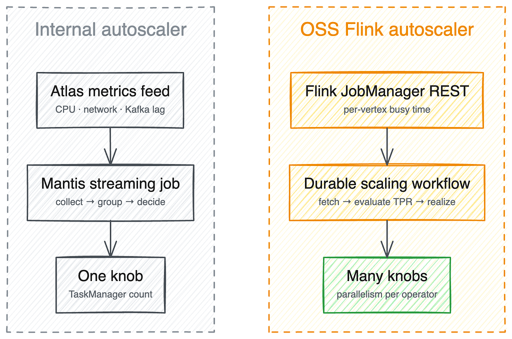
Architecture
Atlas (telemetry) → Mantis (streaming job) → Scaling Decisions
     ↑
External metrics:
- CPU utilization
- Network usage
- Kafka lag
- Input/consume rate
How It Made Decisions
The scaler combined four signals:
- Lag-derived catch-up time — How far behind is the job?
- CPU/network thresholds — Is the cluster under stress?
- Performance history — What has worked before?
- Input rate regression — What is the load trend?
What It Did Well
- Scaled horizontally by adding/removing TaskManagers
- Achieved 25–45% resource reduction across thousands of pipelines
- Scaled itself easily using stream-processing sharding (no custom coordination logic)
- Operated independently of Flink, so Flink issues didn't affect it
Its Critical Limitations
Single knob:  Total TaskManager count
              ↓
All operators scale together
              ↓
Cannot optimize individual bottleneck operators
Two fundamental ceilings:
| Problem | Explanation |
|---|---|
| Coarse visibility | Watched containers from outside — missed internal job behavior |
| Single scaling unit | Entire cluster moved together — couldn't handle multi-operator DAGs |
A Real Failure Example
A networking migration changed how traffic was reported. Some Atlas metrics silently became inaccurate. The gap stayed invisible until it surfaced in production.
This illustrates the danger of depending on external metrics you don't control.
Step 3: The Second Solution — Apache Flink OSS Autoscaler
The Fundamental Difference
Homegrown:  Watches containers from OUTSIDE the job
OSS:        Reasons from INSIDE the job graph
The Key Algorithm — True Processing Rate (TPR)
This is the most important concept to understand.
What Is TPR?
TPR answers: "How much could this operator handle if it were fully busy?"
The Formula
TPR = Observed Throughput / Busy Fraction
Worked Example
Observed throughput:  700 records/sec
Busy fraction:        70% (0.7)

TPR = 700 / 0.7 = 1,000 records/sec
This means the operator could handle 1,000 records/sec at full utilization, even though it's only currently processing 700.
Why This Matters
Flink reports per subtask:
- Time spent doing actual work
- Time spent backpressured (downstream is slow)
- Time spent idle (no data arriving)
By isolating the "busy" fraction, TPR extrapolates true capacity — not just observed load.
How Parallelism Is Calculated
The autoscaler walks the job graph from source to sink:
Source Operator
      ↓
  [TPR calculated]
      ↓
Filter Operator
      ↓
  [TPR calculated]
      ↓
Join Operator  ← Often the bottleneck
      ↓
  [TPR calculated]
      ↓
Sink Operator
For each vertex:
Required Parallelism = Input Rate / (TPR × Target Utilization)
This ensures no single operator becomes a bottleneck while others are over-provisioned.
Side-by-Side Comparison
| Dimension | Homegrown | OSS Autoscaler |
|---|---|---|
| Metric source | External (Atlas/containers) | Internal (Flink JobManager) |
| Scaling unit | Whole cluster | Per operator/vertex |
| Stateful DAG support | ❌ No | ✅ Yes |
| Per-job configuration | ❌ No | ✅ Yes |
| Blind spots | External metric gaps | Requires Flink internals access |
Step 4: Engineering Challenges — From Community to Production
Challenge 1: Integration Without Kubernetes Operator
The OSS autoscaler was originally built inside the Kubernetes Operator for Flink. Netflix doesn't use that operator.
Solution: The community refactored the core into a standalone library with four pluggable interfaces:
┌─────────────────────────────────────────┐
│         OSS Autoscaler Core             │
├──────────────┬──────────────────────────┤
│   Context    │  Job metadata + REST API │
│   State Store│  Persist scaling history │
│ Event Handler│  React to job events     │
│   Realizer   │  Apply scaling decisions │
└──────────────┴──────────────────────────┘
         ↑ Netflix plugs in its own implementations
Challenge 2: Reliability at Scale
First attempt (fragile):
Single batch loop → Job A → Job B → Job C → ...
                              ↑
                    One slow job stalls everything
Solution — Workflow per job (using Temporal):
Orchestrator (polls every ~1 minute)
      ↓
┌─────────────────────────────────────┐
│  Job A Workflow  │  Job B Workflow  │
│  (independent)   │  (independent)   │
└─────────────────────────────────────┘
      ↓                    ↓
Fails/retries alone   Fails/retries alone
Key Principle: Isolate blast radius. One misbehaving job should never affect others.
Challenge 3: Safety Checks Before Scaling
The realizer (the component that applies decisions) runs safety checks first:
Scaling decision made
        ↓
Safety Check 1: Is this region being evacuated? → Block scale-down
Safety Check 2: Is there enough disk for checkpoint state? → Block if not
Safety Check 3: Add standby buffer for large clusters
        ↓
Actuate change through Flink control plane
Step 5: Tuning for Stability — The Target Utilization Trade-off
The Danger of Scaling Too Aggressively
Scale down too far
      ↓
CPU saturates
      ↓
Lag spikes
      ↓
Cannot react instantly (metric window must rebuild after restart)
      ↓
Worse performance than before scaling
Netflix's Conservative Choice
| Setting | Community Default | Netflix Choice |
|---|---|---|
| Target Utilization | 0.70 (70%) | 0.45 (45%) |
Why 0.45?
Lower target utilization
= More headroom before saturation
= Fewer rescales triggered
= More stable large stateful jobs
= Slightly higher cost, but worth it
Trade-off principle: Efficiency and stability are in tension. For large stateful jobs, stability wins.
Step 6: Results and Impact
Quantified Savings
One team's outcome after adopting the OSS autoscaler:
Before: Static provisioning for peak load
After:  Dynamic autoscaling

Result: 58% reduction in compute costs
        ~$1.1 million saved annually
Three Drivers of Savings
1. Daily cycle adaptation
   Peak (weekday) ──────────────────────
   Night/weekend  ─────────
   Autoscaler follows the curve automatically

2. Continuous right-sizing
   No manual intervention after performance improvements
   or post-holiday traffic drops

3. Uniform container dimensions
   Better bin-packing on physical hardware
   More granular scaling increments
Step 7: The Remaining Bottleneck and Future Direction
Current Limitation
Autoscaler logic:  Fast ✅
State recovery:    Slow ❌ (the real bottleneck)
For large stateful jobs, the cost isn't deciding to scale — it's restarting and restoring state.
Flink 2's Solution
Current:  State stored on local disk
          → Rescale requires moving/restoring all state

Flink 2:  Disaggregated state (external storage)
          → Rescale no longer depends on total state size
          → Potentially eliminates recovery bottleneck
Step 8: The Three Generalizable Lessons
These lessons apply beyond Flink to any infrastructure decision:
Lesson 1: External Metrics Have a Ceiling
If you can only see containers, you cannot see operators.
If you cannot see operators, you cannot optimize them.
Principle: Instrument from inside the system you're optimizing.
Lesson 2: Build vs. Buy Is a Moving Target
2019: No mature OSS option → Build
2023: Mature OSS option exists → Adopt

The right answer changes as the ecosystem matures.
Reassess periodically.
Principle: The cost of maintaining custom infrastructure compounds over time. Evaluate regularly.
Lesson 3: Isolation Is a First-Class Design Goal
Shared execution path → Shared failure domain
Per-job workflows    → Isolated failure domain
Principle: Design systems so that one bad actor cannot degrade the whole fleet.
Summary Map
PROBLEM
└── 30,000 jobs, variable load, expensive rescales

SOLUTION 1 (Homegrown, 2019)
├── External metrics (Atlas/Mantis)
├── Single scaling knob (TaskManager count)
├── Works for simple jobs
└── Fails for stateful multi-operator DAGs

SOLUTION 2 (OSS Autoscaler, 2024+)
├── Internal metrics (Flink JobManager)
├── Per-vertex scaling via TPR algorithm
├── Works for complex stateful DAGs
└── Requires integration work for non-standard platforms

KEY ALGORITHM
└── TPR = Throughput / Busy Fraction
    → Parallelism = Input Rate / (TPR × Target Utilization)

KEY ENGINEERING DECISIONS
├── Standalone library (not tied to K8s operator)
├── Workflow-per-job (blast radius isolation)
├── Safety checks before actuation
└── Conservative target utilization (0.45 vs 0.70)

OUTCOME
└── 58% cost reduction, $1.1M saved for one team