Concept 1: What is Document Classification with Large Taxonomies?
The Problem Setup
Imagine you have thousands of documents (product descriptions, medical notes, job postings) and you need to assign each one a label from a massive predefined list called a taxonomy.
Document: "Python developer needed for data pipeline work"
         ↓
Taxonomy: [Software Engineer, Data Scientist, Nurse,
           Accountant, ETL Developer, ... 100,000 more labels]
         ↓
Correct Label: "ETL Developer" or "Software Engineer"
Why it's hard:
- The taxonomy can have 100,000+ labels
- Labels are constantly added, removed, or renamed (taxonomy drift)
- Some labels appear rarely in real data (long-tailed distribution)
- You need it to be accurate, fast, and cheap
Concept 2: Why Traditional Methods Fail
Before modern AI, teams used three approaches — all with serious weaknesses:
Approach 1: Regex / Keyword Matching
Rule: IF document contains "Python" AND "developer" → label = "Software Engineer"
❌ Problem: Breaks on variations like "Pythonista," typos, or new phrasing
Approach 2: Supervised Machine Learning Classifiers
Train a model on labeled examples:
  "nurse needed" → Healthcare
  "code review"  → Software
❌ Problems:
- Needs labeled examples for every label
- Rare labels have too few examples to learn from
- Must retrain every time taxonomy changes
Approach 3: Direct LLM (e.g., GPT, Claude)
Prompt: "Here are 100,000 labels: [label1, label2, ... label100000]
         Which label fits this document?"
❌ Problems:
- 100,000 labels don't fit in the model's context window
- Model starts hallucinating (inventing labels that don't exist)
- Very expensive at scale
Concept 3: Vector Search — The Foundation
This is the first building block of the solution. It converts text into numbers so we can measure meaning similarity.
Step 1: Embeddings
An embedding model converts text into a list of numbers (a vector) that captures meaning:
"Software Engineer" → [0.12, -0.45, 0.78, ... 4096 numbers]
"Code Developer"    → [0.11, -0.43, 0.80, ... 4096 numbers]  ← similar!
"Registered Nurse"  → [-0.34, 0.67, -0.12, ... 4096 numbers] ← different
The article uses Qwen3-Embedding-8B, a top-ranked open model that produces 4096-dimensional vectors.
Step 2: Semantic Score (Cosine Similarity)
Measures the angle between two vectors — closer angle = more similar meaning:
Document vector · Label vector
─────────────────────────────── = cosine similarity (0 to 1)
|Document vector| × |Label vector|

"Python developer" vs "Software Engineer" → 0.89 (high = good match)
"Python developer" vs "Registered Nurse"  → 0.21 (low = poor match)
Step 3: Lexical Score (BM25)
Measures word overlap, but smarter than simple keyword matching:
Shared word "use"  → LOW weight  (appears in thousands of labels, not informative)
Shared word "ETL"  → HIGH weight (rare, very specific and informative)
This is called Inverse Document Frequency (IDF) — rare words matter more.
Step 4: Combining Scores with Reciprocal Rank Fusion (RRF)
Each method produces its own ranked list. RRF merges them by position:
Semantic ranking:  [Label_A #1, Label_C #2, Label_B #3 ...]
Lexical ranking:   [Label_C #1, Label_A #2, Label_D #3 ...]
                              ↓ RRF
Combined ranking:  [Label_A #1, Label_C #2, Label_B #3 ...]
A label ranked highly in both lists gets a strong combined score.
Why Vector Search is Practical at 100k Labels
One-time cost:
  Embed 100k labels → ~1.6 GB storage, ~1-3 minutes
  Build in-memory index → done once per workload

Per-document cost:
  Embed document → find nearest labels → nearly free (CPU ranking)
Concept 4: AI Classify — The Reasoning Layer
Vector search finds candidates. AI Classify picks the winner.
The AI Classify function takes a document and a small set of candidate labels and uses an LLM to reason carefully about which label is the best match:
SELECT AI_CLASSIFY(
  document_text,
  MAP('Software Engineer', 'Designs and builds software systems',
      'ETL Developer',     'Builds data pipelines and transformations',
      'Data Scientist',    'Analyzes data and builds ML models')
) AS predicted_label
Key advantage: It only sees a small shortlist, not 100,000 labels, so:
- No context window overflow
- No hallucination of non-existent labels
- Can reason carefully between similar candidates
Concept 5: The Two-Step Workflow (The Full Solution)
Now combine both concepts into one pipeline:
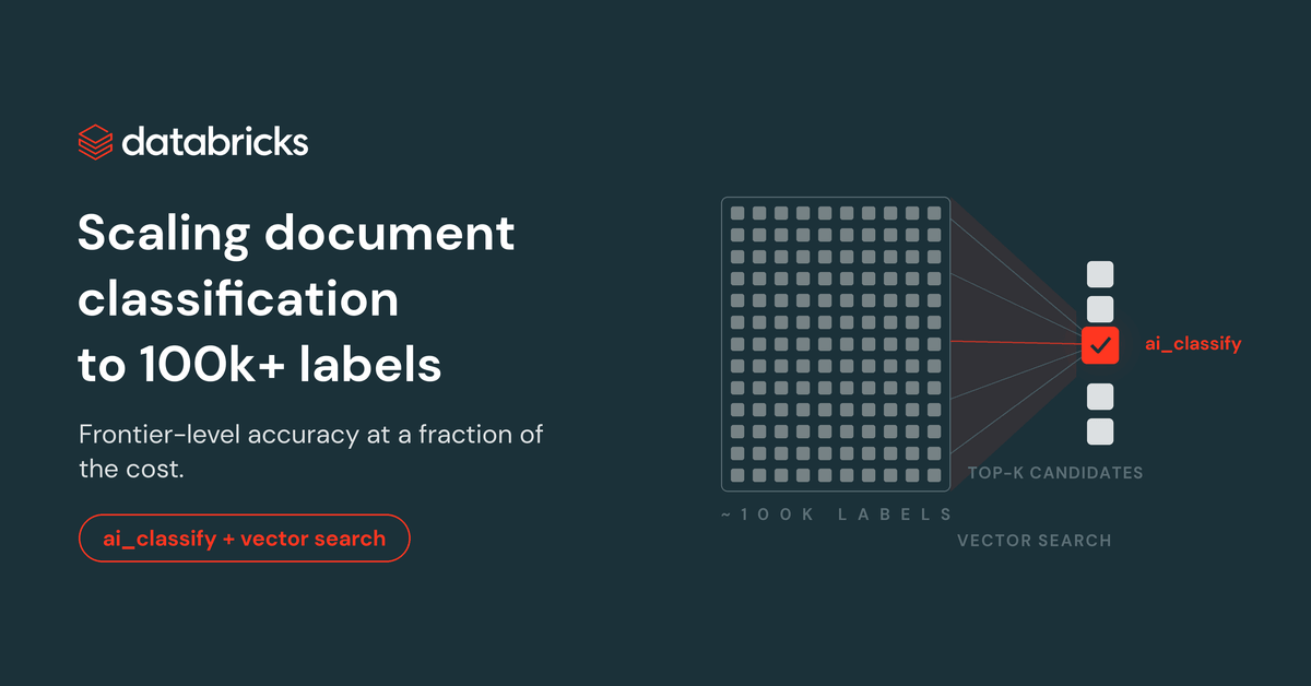
Step 1: VECTOR SEARCH (fast, cheap filtering)
─────────────────────────────────────────────
Document → Embed → Search 100k labels → Top 20 candidates

Step 2: AI CLASSIFY (accurate, focused reasoning)
──────────────────────────────────────────────────
Document + Top 20 candidates → AI Classify → Final label
Choosing K (How Many Candidates to Pass)
The article tested k = 1, 5, 10, 20, 50, 100, 200:
k=1  → Fast but misses the right label often
k=20 → Sweet spot: accuracy stops improving here
k=200→ Slower, more expensive, no accuracy gain
Rule of thumb: Use the smallest k where accuracy plateaus.
Concept 6: Benchmarking — How They Measured Success
Three datasets were tested covering real use cases (35,000 to 100,000 labels).
Metric: Accuracy = fraction of documents where predicted label = correct label
Cost measured: Per-document cost including embeddings + LLM tokens (with prompt caching discounts)
Results Summary
| Method | Accuracy | Relative Cost |
|---|---|---|
| AI Classify Workflow | 0.81 | ~$0.001x |
| Gemini 3.5 Flash (direct) | 0.76 | ~$0.1x |
| GPT-5.4 mini (direct) | ~0.72 | ~$0.05x |
| Vector Search alone | ~0.60 | ~$0.00001x |
AI Classify Workflow vs best frontier model:
  +5 points accuracy
  ~100x cheaper per document
Key insight on large taxonomies: For 100k+ labels, most frontier models couldn't even fit the full taxonomy in their context window. Only GPT-5.6 Luna could — and it still scored below the AI Classify Workflow.
Concept 7: Handling Taxonomy Drift (Ongoing Maintenance)
One of the biggest practical advantages of this approach:
Old approach (classifiers):
  Taxonomy changes → Collect new training data → Retrain model → Redeploy
  Time: Days to weeks

New approach (vector search + AI Classify):
  Taxonomy changes → Remove old label embeddings
                   → Embed new labels
                   → Ingest into index at workflow start
  Time: Minutes
No retraining. No redeployment. Just re-embed the changed labels.
Summary: The Complete Mental Model
PROBLEM: Classify documents into 100k+ labels
         (accurately, cheaply, maintainably)

SOLUTION: Two-step pipeline

┌─────────────────────────────────────────────────────┐
│  ONE-TIME SETUP                                     │
│  Embed all 100k labels → Store in memory index     │
└─────────────────────────────────────────────────────┘
                    ↓
┌─────────────────────────────────────────────────────┐
│  PER DOCUMENT                                       │
│                                                     │
│  Document                                           │
│     ↓                                               │
│  [Step 1] Vector Search                             │
│     Semantic (cosine similarity) +                  │
│     Lexical (BM25) → RRF → Top 20 labels           │
│     ↓                                               │
│  [Step 2] AI Classify                               │
│     Document + Top 20 → LLM reasoning → 1 label    │
└─────────────────────────────────────────────────────┘

RESULT: 81% accuracy, ~100x cheaper than frontier models
        Updates in minutes when taxonomy changes
The core insight is divide and conquer: use cheap vector search to eliminate 99.98% of labels, then use expensive-but-accurate LLM reasoning on only the remaining candidates.