How PID Controllers Coordinate Multiple ML Objectives
Concept 1: The Multitask Conflict Problem
What is it?
When training a machine learning model on multiple objectives simultaneously, those objectives often pull the model in different directions.
How training works (baseline knowledge)
Training Data → Calculate Gradient → Update Model Parameters
                     ↑
              (gradient = direction +
               distance to move in
               parameter space)
The problem with multiple objectives
Imagine three GPS destinations at once:
- Destination A says "turn left"
- Destination B says "turn right"
- Destination C says "go straight"
The standard solution (per-step mixing) averages all directions into one update. This creates three failure modes:
| Failure | What Happens | Why It's Bad |
|---|---|---|
| Disagreement | Conflicting gradients cancel each other | Optimizing one objective hurts another |
| Drift | Objective weights can't adapt fast enough | Outdated objectives still influence training |
| Drought | Adaptive weights shrink some objectives to zero | Can't tell if that objective ever helped |
Key Takeaway
Per-step mixing forces every parameter update to be a compromise, leaving the model suboptimal on all objectives.
Concept 2: Reframing as a Scheduling Problem
The Insight
Instead of asking:
"How do I blend all objectives RIGHT NOW?"
Ask:
"Which objective should get the NEXT block of compute time?"
Why this works
By separating objectives in time rather than blending them simultaneously, you eliminate gradient conflict entirely — objectives never fight over the same update step.
Traditional Mixing:          ControlG Scheduling:
Step 1: A+B+C blended        Block 1: ──── A ────
Step 2: A+B+C blended        Block 2: ──── C ────
Step 3: A+B+C blended        Block 3: ──── B ────
Step 4: A+B+C blended        Block 4: ──── A ────
Proof of concept: Random Scheduling
Even randomly picking which objective gets each block outperforms sophisticated gradient-blending methods:
Random Scheduling avg rank:  5.0  ✓
AutoSSL avg rank:            7.3  ✗
PCGrad avg rank:             7.8  ✗
CAGrad avg rank:             8.4  ✗
Lower rank = better performance
Key Takeaway
Temporal separation alone solves the conflict problem. The remaining challenge is how to schedule intelligently.
Concept 3: The PID Controller — Borrowed from Industry
What is a PID Controller?
A Proportional-Integral-Derivative (PID) controller is a feedback mechanism used in industrial systems to maintain a target state through continuous adjustment.
Real-world examples:
- 🚗 Car cruise control (maintains target speed)
- ☕ Espresso machine (maintains target water temperature)
How PID works conceptually
TARGET ──→ [Compare] ──→ [PID Controller] ──→ [System] ──→ OUTPUT
              ↑                                               |
              └───────────── Feedback ──────────────────────┘
The three terms each handle a different aspect of error:
| Term | What It Corrects | Analogy |
|---|---|---|
| Proportional (P) | Current error (how far off are we now?) | Pressing gas harder when far from target speed |
| Integral (I) | Accumulated past error (persistent bias) | Correcting for a consistent headwind |
| Derivative (D) | Rate of change (prevent overshooting) | Easing off gas as you approach target speed |
Applied to ControlG
The PID controller tracks whether each objective is receiving its planned share of compute:
- P: Prioritize objectives currently behind schedule
- I: Eliminate systematic under-allocation over time
- D: Prevent oscillating between objectives too rapidly
Key Takeaway
PID controllers provide stable, adaptive tracking of a target — here, the target is the planned compute allocation per objective.
Concept 4: Pareto Efficiency in Multiobjective Optimization
What is the Pareto Front?
In multiobjective optimization, the Pareto front is a boundary where:
You cannot improve one objective without making another worse
Objective B
    ↑
    |    × (not Pareto optimal — can improve both)
    |  ●─●─●  ← Pareto Front
    |●         (improving A here requires sacrificing B)
    └──────────→ Objective A
Points on the Pareto front represent the best achievable trade-offs.
Log-Hypervolume: Measuring Distance to the Pareto Front
ControlG uses log-hypervolume to measure how far the current model is from the Pareto front:
Reference Point (current model)
        ↓
   [  gap  ] ← log-hypervolume measures this space
        ↓
   Pareto Front (ideal trade-off boundary)
Log-hypervolume sensitivity answers: "Which objective, if improved, would most increase our distance covered toward the Pareto front?"
This naturally:
- ✅ Prioritizes lagging objectives (those far from optimal)
- ✅ Tempers allocation by how hard each objective is to improve
Key Takeaway
Pareto efficiency gives ControlG a principled way to decide which objective deserves more compute — focus on what's lagging, weighted by difficulty.
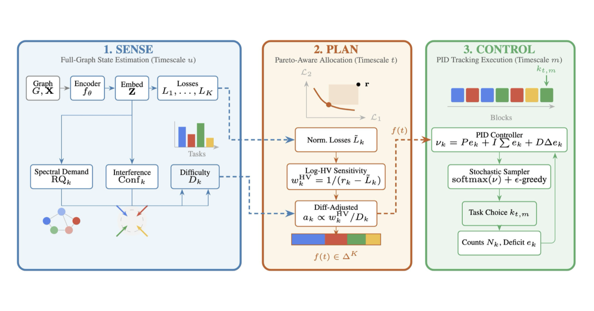
Concept 5: ControlG's Three-Loop Architecture
Overview
ControlG operates at three different time scales, each with a distinct responsibility:
SLOW ──────────────────────────────────────────── FAST
  │                    │                            │
SENSE              PLAN                         CONTROL
(full graph)       (per epoch)                  (per block)
Loop 1: SENSE — Estimating Difficulty
Two signals measure how hard each objective currently is:
Signal A: Spectral Demand
Graph Neural Networks (GNNs) smooth information across neighboring nodes — like blurring nearby pixels in an image.
Node A ──── Node B ──── Node C
  ↓           ↓           ↓
Update↑     Update↓     Update↑   ← Sharp disagreement = HIGH spectral demand
- Smooth objectives: Neighboring nodes want similar updates → easy for GNN
- Sharp objectives: Neighboring nodes want contradictory updates → hard for GNN
Measured formally via the Rayleigh quotient of per-node gradients. This score upper-bounds how much progress one training step can achieve.
Signal B: Interference
How much does optimizing this objective conflict with others?
Uses the Multiple Gradient Descent Algorithm (MGDA) as a measurement tool — it identifies which objectives are currently constraining the Pareto trade-off.
Loop 2: PLAN — Allocating Compute
Combines difficulty estimates with Pareto distance to produce:
Target fraction of compute blocks per objective, per epoch
Objective    Lagging?    Hard?    → Allocation
Link Pred      No         Low     →    15%
Mutual Info    Yes        Medium  →    40%
Reconstruction Yes        High    →    30%
Contrastive    No         Low     →    15%
Loop 3: CONTROL — Executing the Plan
The PID controller tracks actual vs. planned allocation:
Planned allocation: 40% Mutual Info
Actual so far:      30% Mutual Info
Deficit:            10%  → PID increases priority for Mutual Info
The deficit trace is logged and auditable — you can see exactly how well the controller tracked the plan.
Full System Flow
┌─────────────────────────────────────────────────────┐
│  SENSE: Compute spectral demand + interference       │
│         for each objective (slow, full graph)        │
└──────────────────────┬──────────────────────────────┘
                       ↓
┌─────────────────────────────────────────────────────┐
│  PLAN: Use log-hypervolume sensitivity +             │
│        difficulty → target allocation per epoch      │
└──────────────────────┬──────────────────────────────┘
                       ↓
┌─────────────────────────────────────────────────────┐
│  CONTROL: PID controller assigns each compute        │
│           block to one objective, tracks deficit     │
└─────────────────────────────────────────────────────┘
Key Takeaway
The three loops work together: Sense measures reality, Plan sets targets, Control executes faithfully.
Concept 6: Interpretability as a Feature
Why Interpretability Matters
Traditional multitask training is a black box — you can't tell which objective shaped the model or when.
ControlG produces a readable training log:
Early Training:   [A][B][C][D][A][C][B][D]  ← Explores all objectives
Mid Training:     [B][B][B][A][B][B][C][B]  ← Prioritizes Mutual Info (B)
Late Training:    [C][C][A][C][C][D][C][C]  ← Focuses on Reconstruction (C)
What you can audit
| Log Component | What It Shows |
|---|---|
| Scheduling timeline | When each objective received compute |
| Deficit traces | How well PID tracked the plan |
| State trajectories | How difficulty estimates evolved |
Practical value
When a downstream task unexpectedly degrades, the training log reveals which objectives drove the representation and when — enabling diagnosis and correction.
Concept 7: Ablation — Why Each Component Matters
What is ablation?
Removing one component at a time to measure its contribution.
Results
Full ControlG                          → Best performance (baseline)
Remove Planner (uniform allocation)    → Up to -3.4% ← LARGEST drop
Remove both state signals              → Similar large drop
Remove Spectral Demand only            → Drops across ALL graph types
Remove Interference signal only        → Drops most on heterophilic graphs*
Replace PID with random sampling       → -1 to -2%
*Heterophilic graphs = connected nodes have dissimilar features → more cross-task conflict
What this tells us
Component          Role                          Impact if Removed
─────────────────────────────────────────────────────────────────
Planner            Adaptive allocation           Critical (largest drop)
Spectral Demand    Measures GNN difficulty       Universal importance
Interference       Measures cross-task conflict  Critical for conflict-heavy graphs
PID Controller     Accurate plan execution       Moderate but consistent
Summary: The Complete Picture
PROBLEM:  Multiple objectives conflict when blended per-step
             ↓
INSIGHT:  Treat coordination as SCHEDULING, not blending
             ↓
SOLUTION: ControlG's three-loop system

  1. SENSE difficulty (spectral demand + interference)
  2. PLAN allocation (log-hypervolume + difficulty weighting)
  3. CONTROL execution (PID feedback tracking)
             ↓
RESULTS:  Outperforms all baselines, interpretable, efficient
             ↓
BROADER:  Applicable anywhere multiple objectives share
          parameters and conflict over training
Core Principles to Remember
| # | Principle |
|---|---|
| 1 | Gradient conflict is a timing problem, not just a weighting problem |
| 2 | Temporal separation eliminates instantaneous conflict |
| 3 | Adaptive scheduling requires measuring difficulty accurately |
| 4 | Feedback control ensures plans are actually executed |
| 5 | Interpretability is a first-class feature, not an afterthought |